Maps and models often rely on data points collected from the real world—but what happens when there are gaps in the data? Interpolation fills in the blanks, helping you predict unknown values based on the information you do have. But not all interpolation methods are created equal. The right choice can transform incomplete data into powerful, detailed surfaces for analysis and decision-making.
Think of a time you tried to guess a missing number in a sequence or pattern—what clues did you use to make your guess?
A method used to estimate missing values at unknown locations by using patterns found in known data points.
Interpolation is a method used to estimate missing values based on known data points. It works by identifying patterns in the data and using those patterns to predict what’s missing. Take a look at these numbers: 10, 20, 30, ??, 50, 60. What’s missing? You probably guessed 40 (and you’re right, of course) because the numbers follow a predictable pattern. In GIS, interpolation works the same way: It predicts the missing values based on known ones.
Surfaces, like elevation or temperature, often have gaps in the data. To fill these gaps, interpolation methods use patterns in the data to estimate the missing values. Some surfaces change smoothly and steadily, whereas others are more erratic. The method you choose depends on how your data behaves. This lesson walks you through the following three categories of interpolation:
- Linear interpolation: A simple and useful method for smooth surfaces
- Non-linear interpolation: Works well for more realistic and complex data
- Advanced techniques: Best for when you need precision and deeper insights
Check out the sidebar later in this lesson for a cheat sheet on the most common interpolation methods and their best uses.
The word “interpolate” comes from the Latin interpolare, meaning “to polish or refurbish.” In GIS, it’s all about “refurbishing” your data by filling in the missing pieces!
A continuous surface—like elevation, temperature, or rainfall—where values are estimated at every location, even if data was only collected at specific points.
Determining Values with Linear Interpolation
Linear interpolation is the simplest method for estimating missing values. It assumes that your surface changes in a straight line, smoothly and predictably, like a gently sloping hill. Although natural surfaces aren’t usually this perfect, the linear interpolation method lays the groundwork for more complex techniques.
Why do you think linear interpolation is often the first technique taught, even though real-world surfaces are rarely perfectly straight?
Suppose you have two known points:
- Point A is at a 200-foot elevation.
- Point B is at a 400-foot elevation.
- The surface distance between Point A and Point B is 1,000 feet.
You want to estimate the elevation at a point 300 feet from Point A. Here’s how linear interpolation would work:
-
Identify your points: 200 feet at point A and 400 feet at point B.
Estimating elevation at 300 feet from Point A. -
Find the total elevation change:
400 feet – 200 feet = 200 feet -
Divide the total surface distance into equal chunks:
Break 1,000 feet into 10 intervals of 100 feet each.
1,000 feet ÷ 10 = 100 feet per interval -
Calculate the elevation change per interval:
200 feet ÷ 10 = 20 feet per interval -
Estimate the value at 300 feet:
Estimated elevation = (number of intervals × elevation change per interval) + starting elevation-
Number of intervals covered:
300 feet ÷ 100 feet per interval = 3 intervals -
Elevation change:
3 intervals × 20 feet per interval = 60 feet -
Add to Point A’s elevation:
200 feet elevation at Point A + 60 feet = 260 feet
-
Number of intervals covered:
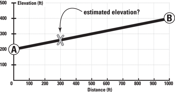

Linear interpolation is great for quick estimates or when you’re working with relatively smooth data. It estimates missing values by assuming a straight line between two known points, dividing the space into equal intervals. The smaller the intervals, the more detailed your results will be, but the values always change at a steady rate—no unexpected jumps or dips.

When using linear interpolation, break the distance into intervals that make sense for your analysis. Large intervals give quick estimates, while smaller ones provide finer detail but require more effort.
Want to go deeper? The science behind linear interpolation
Mathematically, linear interpolation assumes a constant rate of change between two points. The formula for the estimated value at a distance d from Point A is:
Estimated value = Value at A + [(Value at B − Value at A) × (d / total distance)]
This principle underpins many GIS tools, and is the basis for more advanced interpolation techniques like splines and kriging, which add complexity to handle non-linear surfaces.
Where might linear interpolation be misleading when analyzing real-world terrain or weather data?
Linear interpolation always produces accurate results for any type of surface.
Linear interpolation is only accurate for surfaces that change at a constant rate; for more complex or erratic data, more advanced techniques are needed.
City planners use interpolation to estimate air pollution levels at locations where sensors aren’t installed. The method they choose affects how accurately they can identify pollution hotspots and protect public health.
- Understood how interpolation fills gaps in geographic data
- Learned the steps of linear interpolation and how it’s applied
Using Non-linear Interpolation
Not all surfaces follow a straight-line path, especially in the natural world, whose features are more complex. Mountains, rivers, and other natural features often change in irregular ways. For example, a riverbed might gradually deepen before dropping off into a steep canyon, or a city’s temperature might jump abruptly from one block to another due to microclimates. Non-linear interpolation methods are designed to handle these kinds of unpredictable changes by allowing the estimated values to curve, bend, or even spike—just like the natural phenomena they represent.
GIS analysts often start with linear interpolation for a quick look, but switch to non-linear methods like splines or kriging when accuracy matters—for example, in flood modeling or soil property mapping.
Practice linear interpolation using sample data:
- Suppose you have a temperature reading of 15°C at Point C and 25°C at Point D, 500 meters apart.
- Estimate the temperature at a spot 200 meters from Point C using linear interpolation.
- Write down your steps, and check your answer using the formula from this lesson.
What is interpolation in GIS?
Tap to revealIt is a process for estimating unknown values using patterns in known data points.
When is linear interpolation most appropriate?
Tap to revealWhen the underlying data changes smoothly and at a constant rate between points.
What is a statistical surface?
Tap to revealA continuous spatial surface (like elevation or temperature) where values are estimated across the map.
How would your approach to interpolation change if you knew the data had sudden changes or irregularities?
Linear interpolation can accurately predict values for all types of geographic surfaces.
Reflect on a situation—real or hypothetical—where choosing the wrong interpolation method could lead to a critical error in decision-making. What happened, or what could happen, as a result?
Interpolation bridges the gaps in spatial data, but the method you choose—from simple linear to advanced techniques—directly affects the accuracy and usefulness of your geographic analysis.
Linear interpolation is an essential first step for estimating values on smooth surfaces, but recognizing when to use more advanced methods is critical for real-world GIS work.
“It predicts the missing values based on known ones.”